First-order IIR Filter with Simulation

In this example, a direct form first-order IIR filter is designed.

First, we need to import the operations that will be used in the example:

from b_asic.core_operations import ConstantMultiplication
from b_asic.special_operations import Delay, Input, Output

Then, we continue by defining the input and delay element, which we can optionally name.

input = Input(name="My input")
delay = Delay(name="The only delay")

There are a few ways to connect signals. Either explicitly, by instantiating them:

a1 = ConstantMultiplication(0.5, delay)

By operator overloading:

first_addition = a1 + input

Or by creating them, but connecting the input later. Each operation has a function output()).

b1 = ConstantMultiplication(0.7)
b1.input(0).connect(delay)

<b_asic.signal.Signal object at 0x7f5086beea70>

The latter is useful when there is not a single order to create the signal flow graph, e.g., for recursive algorithms. In this example, we could not connect the output of the delay as that was not yet available.

There is also a shorthand form to connect signals using the <<= operator:

delay <<= first_addition

Naturally, it is also possible to write expressions when instantiating operations:

output = Output(b1 + first_addition)

Now, we should create a signal flow graph, but first it must be imported (normally, this should go at the top of the file).

from b_asic.signal_flow_graph import SFG  # noqa: E402

The signal flow graph is defined by its inputs and outputs, so these must be provided. As, in general, there can be multiple inputs and outputs, there should be provided as a list or a tuple.

firstorderiir = SFG([input], [output])

If this is executed in an enriched terminal, such as a Jupyter Notebook, Jupyter QtConsole, or Spyder, just typing the variable name will return a graphical representation of the signal flow graph.

firstorderiir

For now, we can print the precedence relations of the SFG

firstorderiir.print_precedence_graph()

------------------------------------------------------------------------------------------------------------------------
1.1     id: in0,        name: My input,         value: 0,       inputs: {},     outputs: {0: ['add0']}
1.2     id: t0,         name: The only delay,   initial_value: 0,       inputs: {0: ['add0']},  outputs: {0: ['cmul1', 'cmul0']}
------------------------------------------------------------------------------------------------------------------------
2.1     id: cmul1,      name: no_name,  value: 0.7,     inputs: {0: ['t0']},    outputs: {0: ['add1']}
2.2     id: cmul0,      name: no_name,  value: 0.5,     inputs: {0: ['t0']},    outputs: {0: ['add0']}
------------------------------------------------------------------------------------------------------------------------
3.1     id: add0,       name: no_name,  inputs: {0: ['cmul0'], 1: ['in0']},     outputs: {0: ['t0', 'add1']}
------------------------------------------------------------------------------------------------------------------------
4.1     id: add1,       name: no_name,  inputs: {0: ['cmul1'], 1: ['add0']},    outputs: {0: ['out0']}
------------------------------------------------------------------------------------------------------------------------

Executing firstorderiir.precedence_graph will show something like

As seen, each operation has an id, in addition to the optional name. This can be used to access the operation. For example,

firstorderiir.find_by_id('cmul0')

<b_asic.core_operations.ConstantMultiplication object at 0x7f50f4da4d60>

Note that this operation differs from a1 defined above as the operations are copied and recreated once inserted into a signal flow graph.

The signal flow graph can also be simulated. For this, we must import Simulation.

from b_asic.simulation import Simulation  # noqa: E402

The Simulation class require that we provide inputs. These can either be arrays of values or we can use functions that provides the values when provided a time index.

Let us create a simulation that simulates a short impulse response:

sim = Simulation(firstorderiir, [[1, 0, 0, 0, 0]])

To run the simulation for all input samples, we do:

sim.run()

[0.15]

The returned value is the output after the final iteration. However, we may often be interested in the results from the whole simulation. The results from the simulation, which is a dictionary of all the nodes in the signal flow graph, can be obtained as

sim.results

{'add1': array([1.  , 1.2 , 0.6 , 0.3 , 0.15]), 'cmul1': array([0.    , 0.7   , 0.35  , 0.175 , 0.0875]), 't0': array([0.   , 1.   , 0.5  , 0.25 , 0.125]), 'add0': array([1.    , 0.5   , 0.25  , 0.125 , 0.0625]), 'cmul0': array([0.    , 0.5   , 0.25  , 0.125 , 0.0625]), 'in0': array([1, 0, 0, 0, 0]), '0': array([1.  , 1.2 , 0.6 , 0.3 , 0.15])}

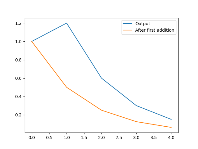
Hence, we can obtain the results that we are interested in and, for example, plot the output and the value after the first addition:

import matplotlib.pyplot as plt  # noqa: E402

plt.plot(sim.results['0'], label="Output")
plt.plot(sim.results['add0'], label="After first addition")
plt.legend()
plt.show()

To compute and plot the frequency response, it is possible to use mplsignal

from mplsignal.freq_plots import freqz_fir  # noqa: E402

freqz_fir(sim.results["0"])
plt.show()

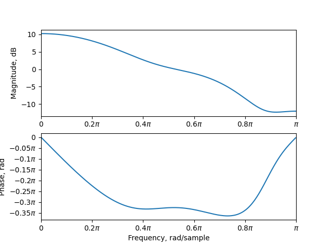
As seen, the output has not converged to zero, leading to that the frequency-response may not be correct, so we want to simulate for a longer time. Instead of just adding zeros to the input array, we can use a function that generates the impulse response instead. There are a number of those defined in B-ASIC for convenience, and the one for an impulse response is called Impulse.

from b_asic.signal_generator import Impulse  # noqa: E402

sim = Simulation(firstorderiir, [Impulse()])

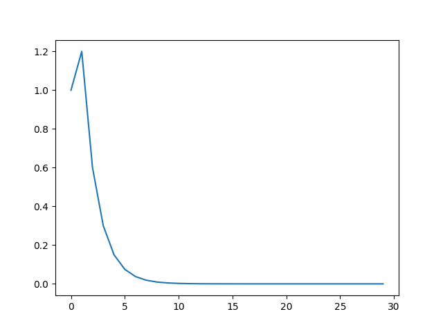
Now, as the functions will not have an end, we must run the simulation for a given number of cycles, say 30. This is done using run_for() instead:

sim.run_for(30)

[4.470348358154297e-09]

Now, plotting the impulse results gives:

plt.plot(sim.results['0'])
plt.show()

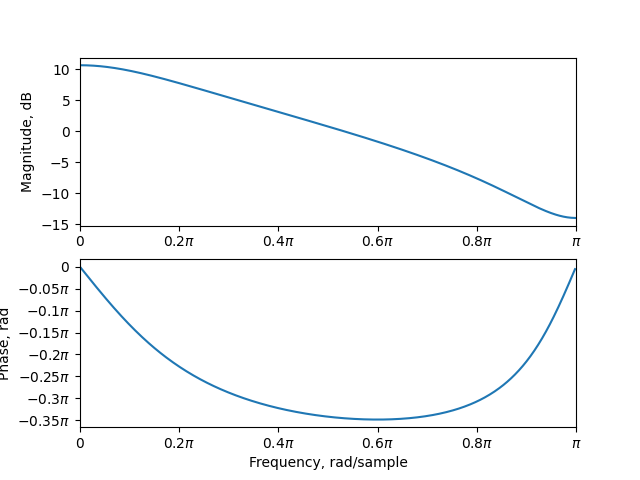
And the frequency-response:

freqz_fir(sim.results["0"])
plt.show()